Beating the NFL Draft: Part Two
Editor’s note: This is the second piece in a three part research paper. Check out part one and be sure to look out for part three.
MODEL BUILDING
Build Space: As mentioned above, the article for the 2008 Pro Football Prospectus was flawed, but the core observation – that a wide receiver’s build, defined by his height and BMI, had predictive power – remained useful as a framework for evaluating WRs.
In fact, it’s important enough that it’s presented here to help understand some of the choices that were made in model building. First, here’s the chart itself:
[am4show have=’g1;’ guest_error=’sub_message’ user_error=’sub_message’ ]
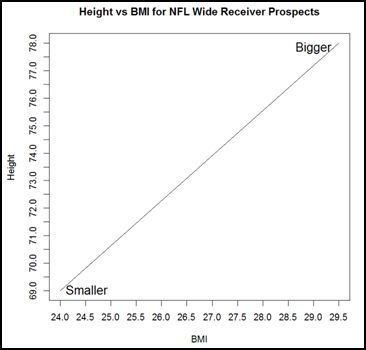
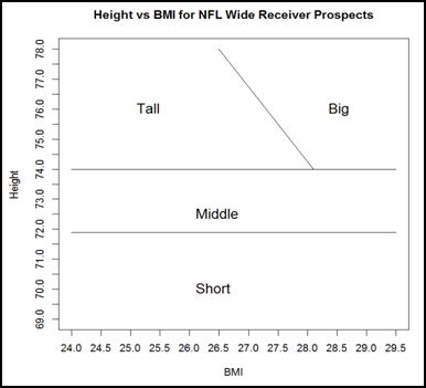
This is what we’ll refer to as the “build space” – an X-Y plane with BMI on the X axis and height on the Y axis, used to visualize a WR’s build. As one moves from the bottom left (short and slight) to the top right (tall and thick) receivers get bigger.
Based on the utility of my naïve models, I believed coming into the practicum project that a WR’s build dominates all other variables. Specifically, I believed three things:
- First, where a WR is located in the build space defines a WR’s type, and that in turn defines what tools are potentially available to him in order to “win” against an opponent. In other words, the variables that are relevant to a WR’s success might be different depending on where he is in the build space.
- Second, even in cases where different build types both used the same variables to “win”, the importance of those relevant variables might change depending on the WR’s location in the build space.
- Third, even though height and BMI are continuous variables, there are discontinuities that act as thresholds between types.
Initial Models: Originally the goal was to beat draft position as a predictor using only other variables – i.e. without including draft position in the models. But in this initial stage of the analysis it quickly became apparent that draft position adds a lot of value not captured in the metrics, with the “metrics only” models performing very poorly.
This makes considerable sense since draft position incorporates a large amount of information not captured in the other measures. A full discussion of those inputs is beyond the scope of this paper, but they can generally be described as psychological, medical, character and work ethic evaluations as well as subjective scouting inputs.
As such the revised goal was to demonstrate that models incorporating both draft position and other metrics can beat draft position alone as a predictor. In other words, to show that the NFL has not historically made full use of the information at its disposal when drafting wide receivers.
In practical terms the models would need an estimate of the player’s draft position in order to make the prediction prior to the draft. However, a rough idea of draft position is often known in advance of the draft so this is not an especially big problem in some cases. Furthermore, even without that knowledge the models could still be used to build a predicted outcomes curve over the possible range where the player might be drafted.
Counter-intuitively, including draft position as a variable in these initial stages yielded information that allowed the subsequent creation of models that in fact do beat draft position without using draft position as an input. That will be covered in the next section.
All of the values reported here will use Root Mean Squared Error (RMSE) as the measure of model performance. RMSE is a standardized way to measure the gap between each of the predicted values and the real world outcomes. It’s the average error of the prediction. So smaller is better – i.e. the gap between the predicted values and the actual values is smaller.
Since the goal here is to beat draft position by itself as a predictor we need to start by obtaining baseline errors for the entire data set – first using the mean of the response variable as our prediction for each record, and then using a bivariate regression using only draft position as an X variable:
- RMSE using the sample mean for every prediction: 66 Adjusted Receiving Yards
- RMSE for a regression using only draft position: 75.73 Adjusted Receiving Yards
The second number, 75.73, is the number we’d like to beat (i.e. the average error is lower than that).
There were four model types developed in the first round of model building:
- Principle Component Analysis and PCA Regression
- Cluster Analysis
- Decision-Trees
- Regression-based models
Since none of these models produced strong results, the detailed discussion of these models has been removed and replaced with a summary table of each method’s performance:
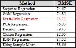
While stepwise regression and some of the other models using local regression did manage to reduce the error relative to draft position by 1%-2% (RMSE of 74.67), none of the models came anywhere close to beating draft position as a predictor by a significant margin. Additionally, the models that I thought might perform best, that seemingly operate most similarly to how I’ve used this data in the past – especially decision trees – fared the worst.
However, I was still convinced that the problem was with my skill as a modeler rather than an absence of the relationships I believed were in the data.
Next Steps and Modeling Breakthrough: As I started writing this report I reviewed these results, and there were a few things that kept me thinking about the problem despite the lack of success. First, a large number of the inflection points in the bivariate regressions were roughly where I expected to find them, and those values are at the heart of the naïve models. Second I was still reasonably confident that what I’d been doing naively for the last few years worked in practice.
After reviewing everything for a few weeks, I thought about how I might create a model that better represented the naïve models. More specifically I wondered if treating each variable as if it represented one continuous measurement was a mistake. My argument coming into the project was that the build space defines receiver type – with relatively sharp height and BMI break points defining the boundaries – and that there were also thresholds or breakpoints in the combine data (speed, explosion, agility) that created discontinuities in NFL performance among otherwise similar WRs.
So, after vetting the idea with two stats professors, the predictor variables were broken into multiple variables, using the inflection points in the exploratory graphs (reproduced here) and previous experience with the data as a guide.


Now, instead of ten predictor variables there were thirty-three:
- logDraft1, logDraft2, logDraft3
- BMI1, BMI2, BMI3
- Age21, Age22, Age23
- VOL1, VOL2, VOL3
- Skill1, Skill2, Skill3
- HT1, HT2, HT3, HT4
- Size1, Size2, Size3, Size4
- SPD1, SPD2, SPD3
- EXP1, EXP2, EXP3
- AGL1, AGL2, AGL3
- Fast
Within the range that defined each of the sub-variables the original, continuous measurement was retained. Outside the range for each sub-variable the variable was simply coded as zero. For example, SPD1 contains all SPD measurements below (-.5), so original values in that range are kept. However anything above (-.5) would be coded as a zero.
The WRs were also divided into four subsets – based on the belief that WRs in different areas of the build space use different physical tools to be successful. The revised build space chart below broadly represents those different WR types. I strongly believe there are further refinements available, but breaking the receivers into smaller subsets creates sample-size problems in terms of proving it statistically.
Subsetting the WRs, breaking up the variables and rerunning a stepwise regression yielded immediate results, as the error reduction improved from roughly 13 (base error of 88.66 to 75.73 for draft position) to a bit over 24 units (88.66 to 64.48) – an 88% lift.
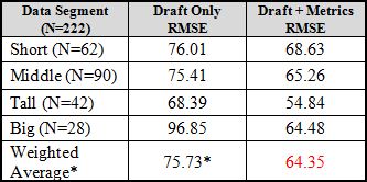
*This total comes from the initial, unsegmented, file. Since it was lower than the weighted average of the segmented data it was used in order to maximize the error reduction provided by draft position.
Check back in tomorrow for the concluding piece.
[/am4show]
- Beating the NFL Draft: Part Three - April 15, 2016
- Beating the NFL Draft: Part Two - April 14, 2016
- Beating the NFL Draft: Part One - April 13, 2016


