Beating the NFL Draft: Part One

By Rob Pitzer

Posted on April 13, 2016

Share

Tweet

Share

Share

Email

Comments

Editor’s note: This is the first piece in a three part research paper. Be sure to look out for parts two and three.

BACKGROUND & INTRODUCTION

This report describes a statistical model that outperforms NFL draft position (from 1999-2011) as a predictor of receiving performance of for NFL wide receivers (WRs), using only quantitative data available at the time of the draft.  With draft position included as in input, the model more than doubles the predictive power of draft position as a stand-alone variable.

The model works by subsetting the WR pool into four “types” based on height and body mass index (BMI), splitting relevant NCAA performance and NFL combine variables into segments, and using piecewise regression on the sub-variables within each WR type.

The results have been cross-validated, reviewed by two statistics professors at George Washington University, and were presented to the department as part of my Masters in Business Analytics practicum project.

By way of background, work on this project began almost a decade ago, and some of the initial ideas on WR build types appeared in a 2008 Pro Football Prospectus article (“Wide Receivers: Size Matters”).  The article itself was largely wrong, or at least very incomplete, but contained some useful ideas that enabled the development of what are referred to in this report as the naïve models – basically the informal findings of the research, iteratively improved on from 2008 until 2014.

In 2014 I chose this research for my practicum project, with the goal of proving what I’d been doing informally was sound, and to discover how much, if any, lift I could achieve relative to draft position.

Based on the success of the WR model presented here there’s reason to believe the same method would work for NFL quarterbacks, running backs and tight ends, however they are not covered in this paper.

 

CONTENTS & ORGANIZATION

[am4show have=’g1;’ guest_error=’sub_message’ user_error=’sub_message’ ]

Data Description

• Records & Original Variables
• Data Sources
• Response Variable: Adjusted Receiving Yards
• Correlations & Variable Reduction
• Exploratory Analysis: Loess Regression Plots
• Final Variables for Analysis

Model Construction

• Build Space: BMI vs Height
• Initial Models & Summary Findings
• Subsequent Models & Breakthrough
  • WR Types
  • Piecewise/Segmented Variables

Discussion of Findings

Post-Practicum Work & Improved Results

• Neural Networks
• Latent Variables
  • Physical
  • Developmental

Limitations of the Research

 

DATA DESCRIPTION

Records:  By far the biggest challenge with this project has been the limited sample sizes.  There are 509 wide receiver prospects in the dataset that are at least partially complete, however:

• 142 are missing data fields required by the models;
• Another 96 entered the NFL between 2012 and 2015, and we don’t have enough data to judge their NFL careers yet (see below);
• 14 played a different position in college and did not catch a pass in college (i.e. they were converted to WR in the NFL);
• 12 records have been removed because the prospect is out of sample either by being too short (below 69”), too thin (below 24.0 BMI) or too slow (slower than 4.79 seconds in the 40 yard dash); and
• One player, Mike Williams, was removed because he was forced to sit out a year between college and the pros – he was ruled ineligible for both his college team and the NFL – after losing a lawsuit against the NFL.

So there are only 222 records available for analysis.

Original Variables:  The original project dataset contained 16 variables:

• Draft Position – a record of where the player was selected in the NFL draft. Each round of the draft has 32 picks and there are 7 rounds, however due to additional picks inserted at the ends of each round from the 3^rd to the 7^th the total number of picks is typically about 250 each year.  Of these, 20-30 will be wide receivers.

• Age – a calculated field using September 1^st of the player’s rookie year minus the player’s DOB, divided by 365.25.

• BCS – a binary variable indicating whether the player attended a big school (a Division-I school) or a smaller school (Division I-AA, Division II or Division III).

• Volume – the number of receptions a player had in his last two years in college.

• Skill – a calculated variable measuring the player’s efficiency with regard to the catches he had in his last two years of college. In simplest terms it considers the result of each a WR’s catches as record, calculates the average result of all his catches, and adjusts the resulting score to account for the influence of other variables.  For example, as volume goes up the raw Skill score falls, on average.  The purpose of this variable is to try and isolate what’s typically described in intangible terms as a player’s “vision”, “field awareness”, “football sense” and the like.  Basically it’s the part of his performance that’s not accounted for by other variables.  After draft position this variable turns out to be the single best predictor of NFL performance.

• Height – the player’s height in inches. Measured to an 8th of an inch at the NFL combine.

• Weight – the player’s weight in pounds. Measured to the nearest pound at the combine.

• BMI – a calculated field using the formula (703 * weight) / (height ^2).

• Size – an interaction effect, weight * BMI. This variable obviously correlates with height, weight and BMI, but, based on previous research, there are areas of the “build space” where size may be more important than weight or BMI.

• 10-yard – the first ten yards of the player’s 40-yard dash time. Timed at the NFL combine to the nearest 1/100th of a second.

• 2nd-10 – the 2nd ten yards of the player’s 40-yard dash time. Timed at the combine to the nearest 1/100th of a second.

• Final 20 – the last 20 yards of the player’s 40-yard dash time. Timed at the combine to the nearest 1/100th of a second.

• Vertical Jump – the height of a player’s standing vertical jump. Measured to ½” at the combine.

• Broad Jump – the player’s standing broad jump. Measured to the nearest inch at the combine.

• 20-yard Shuttle – the player’s time in an agility drill involving two 180 degree changes in direction. Timed at the combine to the nearest 1/100^th of a second.

• 3-cone Drill – the player’s time in an agility drill involving two 180 degree changes of direction and navigation around a set of three cones. Timed at the combine to the nearest 1/100th of a second.

Data Sources and Quality:  The data has been gathered from the Internet.  Age, volume, BCS status, and the collegiate receiving statistics used to create the skill variable are all available prior to the NFL combine from any number of sites.  There are typically no quality or consistency issues with this data.

The performance data is collected during the combine itself.  All of the combine data for this study from the combine is taken from NFL Draft Scout – a scouting service for the NFL, which has prospect data back to 1999 available online.  Additionally, for players who do not participate in the combine, there is often “pro day” data captured during a separate workout – typically on that player’s college campus in the weeks following the combine.

Data from the combine is presumably more reliable due to standard conditions (in the same domed stadium every year) and rigorous procedures for each of the drills.  And in the case of the 40 yard dash there appears to be a “faster” bias in data from pro days.  As a result pro day 40 times have been uniformly increased by .027 seconds in order to match the average time at the combine.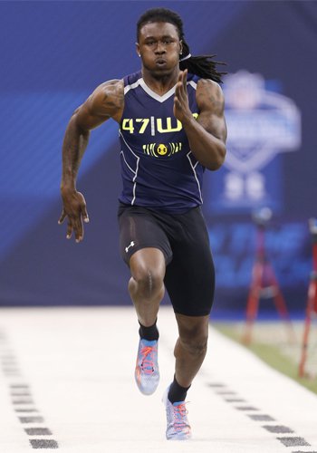

From time to time NFL Draft Scout updates historical data on the 40 yard dash – and it’s not possible to know what’s behind the changes.  However, these updates have resulted in more internally consistent data – for example so that the component times of the 40 yard dash (first 10, second 10, and final 20) are more highly correlated.  The jumps and agility data are not subject to extensive revisions.

Since that data had been collected over time, annually, rather than all at once, the entire file was updated to ensure that the data was current as of Spring, 2014.

While there is unquestionably both measurement and reporting error in the dataset I don’t believe that the errors are systematic.  Additionally, to the extent that they are incorrect they should be, on average, internally consistent relative to one another.  At the very least, they seem to work in the analysis.

Response Variable:  Another data issue was the lack of a natural response variable to use in the analysis.  After some research, I discovered that Neil Payne of 538.com and Chase Stuart at Pro Football Focus had developed a metric to evaluate WRs across time, “True Receiving Yards.”  The starting place for True Receiving Yards is a metric Stuart had previously developed, called “Adjusted Receiving Yards.”  Adjusted Receiving Yards is calculated by taking the total receiving yardage a receiver accumulates during a season, adding five yards per reception and then another 20 yards per touchdown.  The justification for those weights is given in the link above.  It’s possible that using True Receiving Yards would improve these results further, but due to the deadlines of this project, data has not been normalized by either year or team passing yardage.

Having settled on the response variable, an Adjusted Receiving Yards (ARY) measure was generated for every WR season where the WR entered the league after 1998 and had at least one yard receiving/game.  Those totals were then divided by the number of games played each year to get ARY/Game for each player-season.  (Note that the player had to have played at least six of the sixteen games for a season to qualify.)

The total used in the final analysis is the sum of the best two seasons the player had in his first five years as a professional.  Best two of five was chosen to reflect that there is often a multi-season learning curve for new players in the league, many players miss entire seasons due to injury, and using a longer evaluation period (eg, best three of first six years) meant that additional records would be lost.

Once again, there is little doubt that this measure could be improved on, but it seems to be sufficient for an initial effort and produced results that looked right subjectively.  Note that using receiving yards as the basis for the response variable means that the results will only reflect the player’s value as a receiver.  Blocking-first and special teams WRs will have value not accounted for in this analysis.

Correlations and Dimension Reduction:  Because sample size is an issue and some of the combine variables are essentially measuring the same thing, I looked at the correlations to see if some of them could be combined or eliminated prior to model building.  As expected the three segments of the 40-yard dash are correlated (all at .63 or higher), as are the two jumps (.63).  The agility drills are less correlated (.43), but, based on prior use of the data, were also combined.

Those highly-correlated variables were each replaced by a single new variables as follows:

• Speed – the times for the first 10 yards, second 10 yards, final 20 yards of the 40 yard dash were converted to z-scores and the three scores were averaged for each player.
• Explosion – the results of the vertical and broad jumps were converted to z-scores and averaged.
• Agility – the results of the short shuttle and 3-cone agility tests were converted to z-scores and averaged.

BMI and weight are also highly correlated (.85).  However, where weight and height are correlated, BMI and height are not – knowing height tells you next to nothing about BMI (and vice-versa), as demonstrated in the following plots:

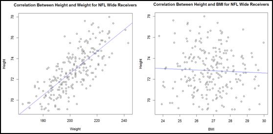
As such, BMI forms one axis of the “build space” that’s at the heart of these models (see below).  Additionally, BMI tested very slightly better as a variable than weight – so weight was dropped as a variable in favor of BMI.

Exploratory Analysis:  Having settled on a data set, finalized the predictor variables, and generated a response variable, simple bivariate plots were generated for all of the predictor variable except BCS (a binary variable) against the response variable.  As a reminder, MaxTYDs2 represents the sum of a player’s best two Adjusted Receiving Yards/Game totals from his first five seasons played – the Y-axis on the graphs below:

Based on these graphs it appears the variables are generally non-linear, and we might suspect that linear methods are not the best choice.  In addition, some of the discontinuities I’d been using in my naïve models were immediately apparent:

• BMI showed clear inflection points at 26 and 28;
• Age also shows a marked slope change at “1” and “2” (representing 22 and 23 years old);
• the lines for explosion and agility are very similar – with a “pause” in the upslope around zero.

Additionally, the “draft” variable looks ripe for a log transformation.  Running the same regression using the transformed variable converts it to a more linear function, so draft was replaced by logDraft) as a variable.

As a result of these changes, the initial variables used in the analysis are:

• logDraft
• Age
• BCS
• Skill
• Height
• BMI
• Size
• Speed
• Explosion
• Agility

Check back in tomorrow, as we continue the analysis.

[/am4show]

Beating the NFL Draft: Part One